Typical Transfer Functions
and their corresponding Frequency Domain Plots

1. First order lag: 

@ low frequency,     LM=0
@ high frequency,  which is a line whose slope is -20 db/decade and an "x-intercept" at w=1/t. @ w=1/t,    LM=-10 log₁₀( 2 )= -3.01 dB @ low frequency,     f=0   @ high frequency,     f= -90^o   @ w=1/t,     f= -45^o    slope= -66^o/decade

  @ low frequency,    LM = 0

@ high frequency,    LM=20 log₁₀( w ) + 20 log₁₀( t )

which is a line whose slope is +20 db/decade and an "x-intercept" at w=1/t. @ w=1/t,  LM=10 log₁₀( 2 )= 3.01 dB   @ low frequency,    f=0^o

@ high frequency,    f=90^o

@ w=1/t, f=45^o    slope= 66^o/decade
 
 

3. Second Order Underdamped Lag: 

@ low frequency,    LM=0
@ high frequency, 

which is a line whose slope is +40 db/decade and an "x-intercept" at w=1/t.

To determine the peak, take derivative of LM with respect to w and then set to zero.

@ low frequency,     f=0^o
@ high frequency,     f=180^o
@ w=1/t,        f=180^o

4. Delay: 

LM=0

@    w=1/t_d f = -57.3^o
@ w=2/td f = -114.6^o
@ w=3/td f = -171.9^o

5. Integrator: 

     : line with a slope = - 20dB/decade

@ w=1     LM=0

5. Differentiator:        G(s) = s
 

        : line with a slope = + 20dB/decade

@ w=1     LM=0

Frequency Plots of Higher Order Transfer Functions

Let    G(s)= G₁(s) G₂(s)

In polar form,

= 

thus,

1)  arg(G) = arg(G₁) + arg(G₂)    or    f = f₁ + f₂
2)    | G | = | G₁ | | G₂ |

In terms of log modulus,

= 

or      LM( G ) = LM( G₁ ) + LM( G₂ )

Implications:

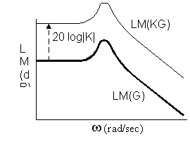
1)    Putting a constant gain K in series with G means | KG | = | K | | G | and

Log modulus plot is translated vertically upward if | K | > 1 (downward if | K | < 1)

Since arg(K)=0, the phase shift vs frequency plot remains unchanged.

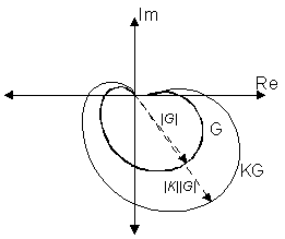
The Nyquist plot expands proportionally away from origin if |K| > 1 ( and shrinks if |K| < 1)

2.     At high frequencies, every polynomial order in the denominator contributes -90^o in the phase shift plot; while every polynomial order in the numerator contributes +90^o.

3.     Using rough line segments for approximate plots, various lead and lags can be combined to produce desired "reshaping" of transfer functions.

Example:

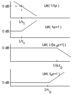
The "real" PID has the transfer function

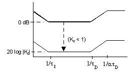
Adding the following log modulus plots:

yields

This page is maintained by Tomas B. Co (tbco@mtu.edu). Last revised 2/10/1999.
     Tomas B. Co
     Associate Professor
     Department of Chemical Engineering
     Michigan Technological University
     1400 Townsend Avenue
     Houghton, MI 49931-1295

Back to Homepage