![]()
in which the output and input variables are in the form of deviation variables.
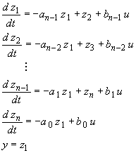
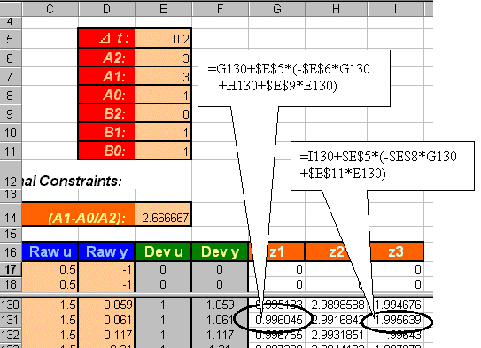
It can be shown that an equivalent system of equations involving only first order derivatives (more easily amenable to Euler integration) is given by
![]()
in which the output and input variables are in the form of deviation variables.
It can be shown that an equivalent system of equations involving only first order derivatives (more easily amenable to Euler integration) is given by

If the input/output data are not yet in the form of deviation variables,
calculate the deviation input/output variables.
If the system is stable, put down additional constraints on the coefficients
of the characteristic polynomial equation: ![]() ,
such that the roots will always have negative real parts.
,
such that the roots will always have negative real parts.
For example, if the polynomial is second order, we need: ![]() .
For a third order system, we need:
.
For a third order system, we need: ![]() .
(These constraints plus other rules for higher order polynomials can be
obtained from the Routh-Hurwitz arrays.) Without violating any of
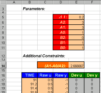
the constraints, enter some initial guesses to the model parameters.
(In this example, we begin with a guess of a2=3, etc. )
.
(These constraints plus other rules for higher order polynomials can be
obtained from the Routh-Hurwitz arrays.) Without violating any of
the constraints, enter some initial guesses to the model parameters.
(In this example, we begin with a guess of a2=3, etc. )
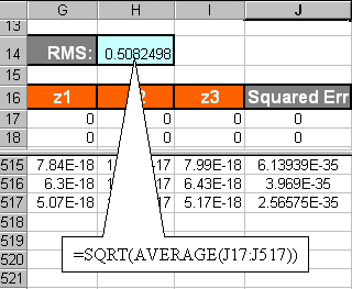
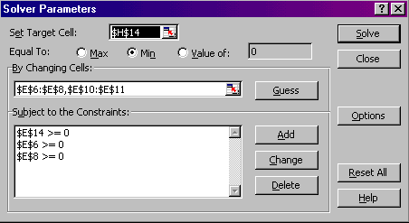
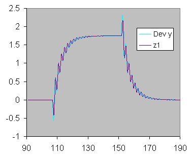
This page is maintained by Tomas B. Co (tbco@mtu.edu). Last revised 1/18/2000.
Tomas B. Co
Associate Professor
Department of Chemical Engineering
Michigan Technological University
1400 Townsend Avenue
Houghton, MI 49931-1295